
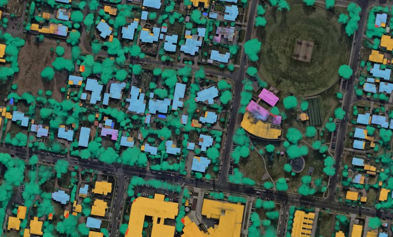
2018 | Flinders Park, Nearmap AI Tree Canopy Boundaries
2018 | Flinders Park, LiDAR 3m Tree Canopy Extent
Post Catastrophe Imagery and AI-derived property damage and condition data unite to help insurers process customer claims more efficiently.
Nearmap AI Tree Canopy Boundaries, Vale Park, early 2018
In the two previous posts, we’ve detailed a 10-year study of Adelaide’s changing tree canopy, from 2011 to 2021. How green is your city?
We covered the city-wide statistics in part 1, and deep-dives on some of the suburbs experiencing greatest change in part 2. One question which has come up since reporting on the study is how Nearmap AI tree canopy compares to LiDAR capture, which has sometimes been referred to as the ‘gold standard’ for mapping tree canopy in cities.
One of the few publicly accessible data sets for tree canopy in Adelaide is a LiDAR study performed across 2018/2019. Specifically, it blends data from two surveys, in April 2018 and October 2019 (18 months apart) into a single data set, and forms the baseline for what we understand will be future analysis. It uses LiDAR classification to map the extent of tree canopy >3m in height.
Below, we show a set of comparisons between the Nearmap AI tree vectors from January–March 2018, which form the foundation of one of the nine individual analysis dates we used in our study, and should be a relatively good temporal match for the data available in the Urban Heat and Tree Mapping Viewer.
High-resolution screenshots of the LiDAR data were spatially-matched to Nearmap data in QGIS using keypoints, so that the reader can flick between the two.
NB: The backing imagery used for the separate LiDAR study is more recent (appears to be ~2021), and lower-resolution and should be ignored for that reason.
While only a qualitative comparison is possible with visual inspection, we suggest there are four things to look out for:
You may wonder: “were these locations picked to show Nearmap data in a favourable light”? The answer here is ‘no’. I chose one location with very dense tree cover, one typical suburban tree cover, and one with some smaller, more intricately structured patterns of suburban trees. I encourage you to browse the Mapping Viewer to look at the LiDAR data, and the many examples of Nearmap AI tree data online and reported in media (or contact us to request a demo). My best judgement is that these findings would be consistent in any set of examples from this Adelaide survey. The main bias is that the comparison of a decade of Nearmap AI data is compared with one single LiDAR capture. Different companies with different sensors and processing systems may also arrive at different results.
Applying the qualitative comparison criteria above, we can observe:
1. Systematic differences: For both the smaller trees and larger clumps of tree cover, it appears that the boundary area is similar enough that they fall within ‘visual tolerance’. It is likely there is some systematic difference, as any two different methodologies will have, but it is small enough to require proper quantitative analysis to detect. Specifically addressing the 2m vs 3m definition question, this does not seem to be an issue. With a range of tree heights, there are only two or three small trees that Nearmap includes, that the LiDAR excludes. By contrast, there are perhaps five or six small trees that the LiDAR includes, but Nearmap AI ignores. If the definitional difference of 2m for Nearmap was key, one would expect this to be the other way around (Nearmap including small trees in the 2-3m height range that are rejected by the LiDAR data). This reversed result implies that the methodological differences between the two approaches (deep learning on imagery vs laser reflectance) are more important for which trees are included, than the subtle definitional distinction between a 2m or 3m minimum tree height.
2. Artefacts: LiDAR starts as a point cloud, but then requires subsequent processing to produce a vector map on which to compute tree canopy cover. The documentation linked from the Urban Heat and Tree Mapping Viewer describes it as 8 points per square metre, and processed to a 1 by 1 metre grid. By contrast, Nearmap AI data is fundamentally computed at 7.5cm/pixel (roughly speaking 170 dots per square metre), with vectorisation and smoothing applied in post-processing. This results in the somewhat jagged appearance of the LiDAR in 1x1m grid cells, compared to smoother Nearmap AI outlines. Further, because the Nearmap AI model uses deep-learning to identify tree and other classes by simultaneously considering all image pixels in a large context area, it does not exhibit the same small holes and patchiness apparent in LiDAR processed data. That said, both of these issues are largely aesthetic, and are unlikely to impact a measure such as suburb-level (or even mesh block) tree canopy cover.
3 & 4. False positives/negatives: Neither image appears to include significant false positives or negatives, with the exception that some smaller trees, potentially only a few metres tall, show a level of disagreement in the data set. While “boots on the ground” verification could clear this up, the difference seems insignificant for tree canopy analysis. One would then have to consider whether, for example, a single branch poking above the rest is sufficient to classify as tree or not tree.
Let’s quickly revisit the points above, noting anything new in this example:
1. Systematic Differences: The LiDAR, perhaps due to the lower resolution, possibly has a little systematic bias to over predict when two trees are linked. Where the Nearmap AI results tuck in around individual trees more tightly, the LiDAR tends to link them with a thicker band. This is a barely noticeable effect though, and unlikely to impact tree canopy results.
2. Artefacts: There’s a fascinating LiDAR artefact with the group of trees in the centre, likely caused by aggregation to 1 sqm grid cells.
3 & 4. False Positives/Negatives: Once again, there are some disagreements on smaller trees, but more balanced in this image. This means the total tree cover is unlikely to differ significantly.
For the final example, there are no additional points of great interest – just another image to reinforce the above conclusions.
The above comparisons show a good visual sense of how the two data sets behave. While this is not a quantitative comparison, it is clear that both methodologies capture tree cover with a high degree of accuracy. Summarising the major differences:
Both data sets appear to be useful and valid in determining extent of tree canopy in residential areas. However, there will be methodological biases that are too subtle to detect visually. The most crucial thing in assessing change between dates is that a consistent methodology is used (LiDAR vs LiDAR change with the same setup, or Nearmap AI vs Nearmap AI). In areas where the true change are small, it is critical that a methodologically caused systematic difference is not mistaken for a genuine change in tree cover.
If both methodologies provide good quality tree cover measures, the question of scale and frequency becomes important. Due to the high cost, LiDAR surveys are often flown on restricted areas, and rarely on an annual basis. By contrast, Nearmap AI vegetation maps are produced up to six times per year in Adelaide, with over 85 aerial imagery captures between 2009 and 2022 that can have Nearmap AI applied to them (although we recommend seasonally-matched comparisons for optimal results – e.g. summer to summer). Having many time points to work with becomes a hugely valuable asset for comparing long and short range change, looking at trends (and how the trends are changing over time), and predicting future tree change based on a number of recent data points. If the aim is to make adjustments to behaviour and policy, and then observe the impact of those changes as quickly as possible, it is important to take frequent (at least annual) measurements, and observe whether the trend over previous years has changed.
Further, the fact that Nearmap AI vegetation maps are produced using an identical methodology across hundreds of urban areas in four countries means that both longitudinal and spatial comparisons can be made in a valid way.
We haven’t yet covered 3D structure. LiDAR certainly can provide excellent information about the 3D structure of trees, and can be used for estimating things such as biomass, tree height, etc. The comparison above focuses solely on usefulness for this study: to measure the extent of changes in tree canopy. Nearmap 3D can be combined with Nearmap AI to capture information such as vegetation heights. I won’t comment on a comparison to LiDAR here, as it was beyond the scope of this study – other than to say that I know it works, and have seen it done in practice.
The last comparison point is that often tree canopy change, particularly measured over time, is ideally done with other features as well. Perhaps the goal is to study the relationship between a rise in buildings, asphalt areas, construction, or other features. “Building footprint” was the only other feature used here (shown in the suburb graphs in the last post), which was a deliberate effort to maintain simplicity. This study is intended to show the power of what can be done with just two feature classes. In reality, there are dozens of distinct feature classes all produced by the same deep learning model, on exactly the same imagery, that form the Nearmap AI product suite, and a plethora of investigations waiting to be conducted. There is very high value in having spatially registered, temporally identical features, available on the same spatial extent and scale. Combining multiple data sets with partially overlapping coverage, at mismatching time points and the like can be very challenging, and the results are open to question.
There are different approaches for tree canopy mapping. I trust that the above comparisons show equivalent and comparable quality is achieved when comparing Nearmap AI with LiDAR.
When combined with Nearmap AI tree canopy, its abundant availability (scale, frequency and currency) and richness of other available features, I’m convinced it will be a game changer in the management of urban forests.
Deep-diving on the history of a single city proved to be a fascinating journey, with some compelling results. We explored from a high level, and aggregated statistics about city-wide changes. We uncovered the stories of individual suburbs, including inspecting individual trees – which have grown and which have been removed. An integrated analysis methodology like this offers a single source of truth for a wide variety of purposes – from city planning, to understanding what has been happening in a single street, and making the data accessible to anyone willing to put eyes on an actual aerial image.
The multiple time points provided far more information than a simple two-date comparison. We were able to identify events at particular times in a suburb’s history, and, based on the most recent few years, whether a trend is likely to continue. The noise level (random fluctuations between years) was sufficiently small that it rarely compromised the comparison from one year to the next. Fluctuations were also negligible in the face of a full decade of accumulated changes.
Finally, while the focus here was on Adelaide, the Nearmap capture program, visual and artificial intelligence products mean that this study is possible to repeat in any of the hundreds of urban areas covered by the Nearmap capture program in four countries, and valid comparisons may be drawn due to the consistently applied methodology.
We’ll be curious to see what comes of this work, and are eager to collaborate with organisations that want to understand where tree canopy (and our dozens of other AI derived layers) in their area of interest has been in the past, and want to work together to actively monitor how they are shaped in future.
-----
Some LGAs list the same suburb as both the 'greenest suburb' and 'least green suburb'. This means that there was only a single residential suburb within the LGA fully covered by the analysis.
Nearmap does not warrant or accept any liability in relation to the accuracy, correctness or reliability of the data provided as part of the Nearmap Leafiest Suburbs analysis. The Nearmap Leafiest Suburbs analysis is based on Nearmap AI data, which detects trees approximately 2m or higher. The national aerial data was collected Oct 2020-March 2021. Results were aggregated at mesh block level using the 2021 Australian Bureau of Statistics definitions. Approximately 5,000 suburbs were included in the analysis, where Nearmap AI coverage exceeded 99%. The top suburbs are those with the greatest percent tree cover in each 2021 SA4 region, and where there is a minimum population of 1,000 residents (2016 census). For suburbs that span multiple LGAs, that suburb is assigned to the LGA that contains the highest proportion of that suburb’s area. City-based metrics analyse all Nearmap AI covered suburbs within the relevant ABS GCCSA region. For the capital city suburb breakdowns, we also refined the analysis to only include ‘residential’ mesh blocks. All percentage figures have been rounded to the closest whole number.
------
About the author:
With degrees in electrical engineering and physics — and a passion for machine learning — Dr Michael Bewley joined Nearmap in 2017 as our first data scientist. Now the Senior Director of AI Systems, he leads the development of the Nearmap artificial intelligence product suite, quantifying the evolution of cities with the most superior AI data sets.
* 281 suburbs within greater Adelaide were included in the analysis, where Nearmap AI coverage exceeded 99%. The analysis includes each suburb where there is a minimum population of 1,000 residents (2016 census).
Analysis fundamentals
The fundamental aspects of the national study were reused for consistency. Key points include:
While we make every effort to ensure the accuracy of the data and analysis in blog articles, this information is not to be relied on as professional advice. No endorsement or approval of any third parties or their advice, opinions, information, products or services is expressed or implied by any information in the blog. Should you seek to rely in any way whatsoever upon this content, you do so at your own risk.